Cross-Entropy Loss

What exactly is cross-entropy loss?

In this post, I’ll discuss what I’ve learnt about the intuition behind cross-entropy loss. This was heavily inspired by Chapter 7 of Stanford’s Speech and Language Processing textbook, and Adian Liusie’s video on the topic.

What is cross-entropy loss?

From Wikipedia:

In information theory, the cross-entropy between two probability distributions p and q , over the same underlying set of events, measures the average number of bits needed to identify an event drawn from the set when the coding scheme used for the set is optimized for an estimated probability distribution q , rather than the true distribution p .

Essentially, cross-entropy loss is used to measure the difference between the model’s predicted probabilities and the actual probabilities. The higher the cross-entropy loss, the greater the difference between your model’s predictions and the actual probabilities. Thus, cross-entropy loss is known as a loss function which we minimise in machine learning through backpropagation in order to build models with higher accuracies.

The basis of cross-entropy loss

Cross-entropy loss is based on Kullback-Leibler (KL) divergence, which is a measure from information theory that measures the difference between probability distributions.

Let’s say we had 2 coins,

$Coin 1=\begin{cases}p1 & heads\\ p2 & tails\end{cases}$

$Coin 2=\begin{cases}q1 & heads\\ q2 & tails\end{cases}$

For example, if our sequence was HTHHTTH, we get $p1\cdot p2\cdot p1\cdot p1\cdot p2\cdot p2\cdot p1$ and $q1\cdot q2\cdot q1\cdot q1\cdot q2\cdot q2\cdot q1$ for Coin 1 and 2 respectively.

Simplifying, we get $p_1^{N_H} \, {p_2^{N_T}}$ and $q_1^{N_H} \, {q_2^{N_T}}$, where $N_H$ is the number of heads and $N_T$ is the number of tails.

Let’s calculate the ratios of the likelihood of observations of each coin: $\dfrac{P(\text{Observations} \mid \text{coin 1})}{P(\text{Observations} \mid \text{coin 2})} = \dfrac{p_1^{N_H} \, p_2^{N_T}}{q_1^{N_H} \, q_2^{N_T}}$

To normalize for the number of samples, let’s take that to the power of 1/N, so that when we log we get:

$\dfrac{1}{N} \log(\dfrac{p_1^{N_H} \, p_2^{N_T}}{q_1^{N_H} \, q_2^{N_T}})$

Expanding, we get:

$\dfrac{1}{N}log(p1^{N_H}) + \dfrac{1}{N}log(p2^{N_T})+\dfrac{1}{N}log(q1^{N_H})+\dfrac{1}{N}log(q2^{N_T})$

Which simplifies to:

$\dfrac{N_H}{N}log(p1) + \dfrac{N_T}{N}log(p2)-\dfrac{N_H}{N}log(q1)-\dfrac{N_T}{N}log(q2)$

If the observations are generated by coin 1, as the observations grow to infinity, the expected proportion of heads will tend to $p_1$ and the proportion of tails will tend to $p_2$. By taking the limit, $\dfrac{N_H}{N}$ becomes $p1$ and $\dfrac{N_T}{N}$ becomes $p2$.

Thus we can further simplify to

$p_1log(p1) + p_2log(p2)-p_1log(q1)-p_2log(q2)$

Which then becomes

$p_1log(\dfrac{p_1}{q_1}) + p_2log(\dfrac{p_2}{q_2})$

And that’s the KL Divergence!

$KL(P||Q)=\sum_{x}P(x)\log(\frac{P(x)}{Q(x)})$

Deriving cross-entropy loss

In a machine learning classification task, we have a list of possible classes and the respective probabilities, giving a probability distribution.

Let the input image be $x_i$ and the predicted class distribution is $P(y|x_i;\theta)$, where $\theta$ is the model’s parameters. The true class distribution is $P^*(y|x_i)$.

Now we want to apply the KL Divergence (explained above):

$KL(P*||P)=\sum_{y}P^*(y|x_i)\log(\frac{P^*(y|x_i)}{P(y|x_i;\theta)})$

$KL(P*||P)=\sum_{y}P^*(y|x_i)[\log({P^*(y|x_i)}-{P(y|x_i;\theta)})]$

$KL(P*||P)=\sum_{y}P^*(y|x_i)\log({P^*(y|x_i)}- \sum_{y}P^*(y|x_i)\log{P(y|x_i;\theta)})$

Notice that the first term doesn’t depend on $\theta$, the model’s parameters. So if we want to minimise this with respect to the model’s parameters, it’s the same as only minimising the second term $- \sum_{y}P^*(y|x_i)\log{P(y|x_i;\theta)})$

And that’s the formula for cross-entropy loss!

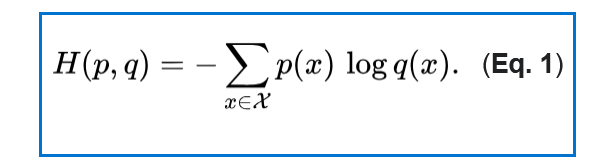Cross-Entropy Loss Formula

Conclusion

Cross-entropy loss is a very popular loss function used in multi-class classification problems. It’s a highly intuitive way of finding the difference between probability distributions. Hope that this article was useful!